Report about the Course on Genomic Selection in Davos in June 2011

Report about the Course on Genomic Selection in Davos in June 2011

by Nicola Bacciu, Alex Barenco, Anna Bieber and Farhad Vahidi

From June 20-24, 2011 a course on genomic selection, one of the LowInputBreeds specialist training workshops, took place in Davos, Switzerland. It was organized by LowInputBreeds partner agn Genetics, together with the Animal Breeding and Genomics Centre and the Wageningen Institute of Animal Sciences from Wageningen University and Research Centre.
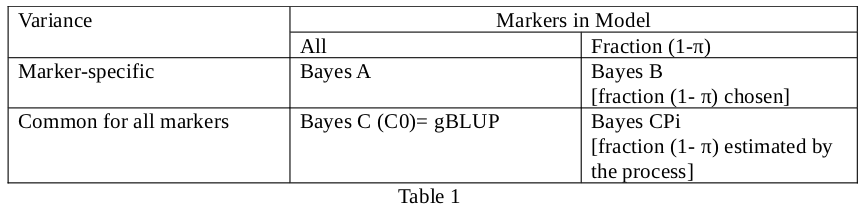
The aim of the course was the estimation of marker effects (in this case SNPs) for genomic selection. Phenotypic data and Single Nucleotide Polymorphism (SNP) genotypes were analysed with mixed linear models solved by Least Squares or Bayesian Methods. Bayesian methods (A, B, C and CPi) were explained. The course was given Prof. Dr. Dorian Garrick and Professor Dr. Rohan Fernando, both from the Department of Animal Science, Iowa State University, USA.

Some properties of these methods are outlined in Table 1.

On the first day, Prof. Dr. Garrick explained the principles of the traditional genetic evaluation based on Henderson's Mixed Model Equation (MME). Based on SNP data, the covariance between relatives can be estimated more accurately for specific chromosomal segments than by the average relationship atrix A. In laboratory 1, exercises were done using the statistical software R to better understand the programming language and mixed linear modelling.

Prof. Dr. Fernando introduced the general concept of Bayesian analysis, using the Bayes Theorem. Conditional, joint and marginal probabilities were introduced and prior belief, likelihood and posterior distribution explained.
In Bayesian statistics probabilities are used to quantify beliefs or knowledge about possible values of parameters.

Three steps of Bayesian data analysis can be distinguished:

1. Setting up a full probability model: provide a joint probability distribution for all variables
2. Calculating and interpreting the appropriate posterior (conditional probability distribution) using prior beliefs and observed data
3. Evaluating the fit of the model and implication of the posterior distribution

One of the main differences between classical and Bayesian statistics is the integration of prior information. Hereby beliefs about parameters are assumed previously to data analysis and formulated as prior probabilities. The evidence from the trial/data set is described using a so-called likelihood function. The likelihood is the conditional probability for the data given the parameters. Combining the prior assumptions and the likelihood function leads to the so-called posterior probabilities, which are conditional probabilities for the parameters given the data.

In the laboratory work, a small example of a Gibbs sampler was derived to generate samples from a normal distribution. Gibbs sampling is one of the simpler Markov chain Monte Carlo (MCMC) algorithms. Among other applications it is a common method to approximate the joint distribution for all variables.
On the second day, Prof. Dr. Rohan Fernando, , extended the Gibbs sampler to a Metropolis Hastings sampler or (also belonging to the MCMC algorithms) which is used to sample from the variables if distribution is not easily sampled. In our case the concept of sampling from a proposal distribution was introduced.

Professor Garrick explained the two steps of genomic evaluation (estimating SNP effects and prediction of genotypic values). He introduced the fixed effect model in various parameterizations (allelic vs. genotypic).

He introduced random effect models to fit allele or substitution effects and showed that the models do not have the same assumptions. However it is straightforward to calculate allele effects from substitution effects and vice versa. Exercises to better understand and use those methods were done in R.
Afterwards, problems due to incomplete linkage disequilibrium (LD) between markers and Quantitative Trait Loci (QTL) and due to fewer observations than the number of marker effects to estimate were explained. Professor Fernando showed the application of Bayesian methods to estimate SNP effects by assuming the SNP effects to be sampled form a single normal distribution. When all SNPs are fitted, this is usually referred to as GBLUP.

On the fourth day, Bayes A was introduced by Professor Fernando, i.e. sampling the SNP effects from a univariate distributionwith only one random variable. An example Bayes A program was given to us in R, permitting us to better understand the sampling process. With some minor changes in the calculation of variances for the Bayes A program, it was possible to create an R program performing Bayes C analyses. Afterwards, the Bayes B method was introduced and some applications were shown by Professor Fernando.

On day 5, Professor Fernandez explained for Bayes C how the fraction of markers in the model can be estimated from the data (Bayes Cπ). Professor Garrick explained the concept of shrinkage estimators using results from Bayes C (GBLUP), Bayes A and Bayes Cπ. At last Professor Garrick gave some advice about the interpretation of results of genome-wide genetic analyses, related problems and challenges in practical situations. Specifically, he elaborated on the fact that SNP effects are capturing covariance between relatives in the absence of sufficient linkage disequilibrium (LD) between markers and (unknown) Quantitative Trait Loci (QTL). Furthermore, he introduced challenges when high density SNP information is imputed from low density genotyping.

Links

• Wikipedia.org: Single-nucleotide polymorphism
• Wikipedia.org: Bayesian probability